Data Blending in Looker Studio: Joins, Metrics and the Traps in Between

Data Blending is the feature in Looker Studio, formerly Data Studio, that combines several data sources in one chart. It is also the feature that produces the most confidently wrong numbers, because a blend fails quietly: the report renders, the totals look plausible, and nothing indicates that a figure has been counted three times or that two de-duplicated counts have been added together as if they were quantities.

The reason is that a blend does not behave like a spreadsheet lookup. Understanding the order in which it works explains almost every strange result, so that is where this starts.

What a Blend Actually Does

A blend performs two operations, in this order: each table is aggregated on its own dimensions first, and the aggregated results are joined afterwards on the configured key. Both halves of that sentence matter. The aggregation happens before the join, so the dimensions chosen for a table determine how many rows that table brings into the join — and the join then matches those rows against the other table, row by row.

This is why a blend is not a lookup and why the choice of dimensions is not cosmetic. Adding a dimension to one table does not simply add a column; it changes the number of rows that table contributes, and therefore what the join produces.

The Five Join Types

Looker Studio offers the standard set, and the choice decides which rows survive when a key exists on one side only:

• Left outer — every row of the left table, plus matching rows from the right. Unmatched right-side rows are discarded. The default, and the reason a date on which only the second source had activity can vanish from a report.
• Right outer — the mirror image; rarely the clearest way to express an intention, since reordering the tables and using a left join usually reads better.
• Inner — only keys present in both tables. Useful when a row is only meaningful if both sources have data, and dangerous when that is not actually true.
• Full outer — every row from both sides, matched where possible. The safest choice when completeness matters more than compactness, at the cost of null-heavy rows that calculated fields have to handle.
• Cross — every row combined with every row. Legitimate for building a scaffold, such as pairing a date list with a channel list, and catastrophic if selected by accident.

A practical rule: when the question is “how did these two things develop over the same period”, full outer on the date protects against silently dropped days. When the question is “what happened to the records that exist in both systems”, inner is the honest choice — but the count of rows it removes is itself worth reporting.

Where Join Keys Break Without Warning

A join key has to match exactly, and most failures come from values that look identical to a reader and are not identical to the machine.

Date granularity is the most common: one source delivering a date-time and the other a date will never match, and the fix is to expose a plain date field in each source rather than to hope the blend reconciles them. Case and whitespace are next — Newsletter, newsletter and newsletter  are three different keys. Normalising with LOWER() and TRIM() belongs in the data source as a calculated field, because a field created there is available as a join key, whereas the blend editor is not the right place to be repairing input data. Currency and locale formatting cause the same class of failure on numeric or identifier keys.

One further constraint is structural: keys with very high cardinality, such as a transaction id, make blends slow, and a blend that times out is a blank chart rather than an error message.

Dimensions Decide What One Row Means

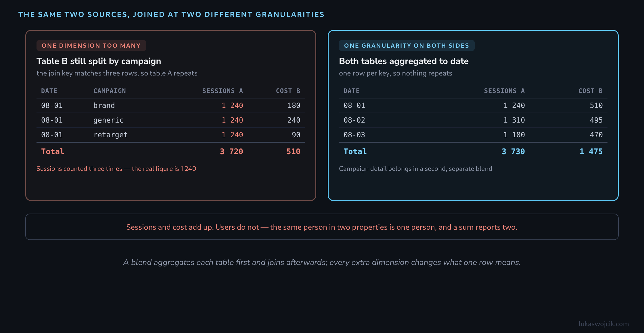
The single most expensive mistake is leaving a dimension in one table that the other does not have. If table A is aggregated by date and table B by date and campaign, the join key of date matches one row of A against three rows of B, and A’s metric is repeated three times. The total is then exactly three times too large — and it is still a round, plausible-looking figure.

Two habits prevent it. The first is to decide the granularity of the blend before choosing any field, and to aggregate every table to exactly that granularity — if the blend is at date level, no table carries campaign. The second is a diagnostic: adding Record Count from each table into a temporary table view shows immediately whether a key is matching more rows than expected, since a clean one-to-one join returns a record count of one per row per table.

Where campaign-level detail is genuinely needed, it belongs in a second blend built at that granularity, not in the same one. A single blend serving two granularities is the request that cannot be satisfied.

Metric Names and Sums Across Properties

Combining the same metric from several properties — total users from three regional GA4 properties, for instance — runs into a behaviour that is easy to mistake for a calculation error.

Every table in a blend keeps its source field names. When three tables each contribute a field called Total users, three fields with the same name enter the blend, and a calculated field written as an addition of that name has no unambiguous way to bind to the right one. What follows is a number that is produced without an error message and is not the intended sum.

The fix is to rename each metric inside the blend editor before writing any calculated field. Giving them explicit, distinct names — users_de, users_at, users_ch — makes the reference unambiguous, and the addition then behaves:

-- Only reliable once each source metric carries a unique name
users_de + users_at + users_ch

Worth checking in the same pass: the aggregation set on each metric in the blend. A field arriving with automatic aggregation can behave differently from one explicitly set to SUM, and since both render without complaint, the explicit setting is the one to prefer.

Metrics That Must Not Be Summed at All

Renaming makes the addition work mechanically. Whether the addition means anything is a separate question, and for two categories of metric the answer is no.

De-duplicated counts — users, active users, any distinct count — are not additive. A person visiting two of the three properties is one person; adding the three counts reports two. The same applies across time: summing daily users across a month does not produce monthly users. There is no blend configuration that fixes this, because the information needed to de-duplicate is not present in the aggregated figures. Where a genuine cross-property user count is required, the data has to be de-duplicated before it reaches Looker Studio, which in practice means the underlying event data in a warehouse.

Rates and averages — CTR, conversion rate, bounce rate, average order value — must be recomputed after the blend rather than combined. The average of two conversion rates is not the conversion rate of the combined data unless both sides happen to have identical denominators. The correct form sums the components and divides at the end:

-- Wrong: averaging two rates
(conv_rate_a + conv_rate_b) / 2

-- Right: recompute from the summed components
(conversions_a + conversions_b) / (sessions_a + sessions_b)

Further Techniques Worth Knowing

• A calendar table as the anchor. Blending both sources against a small table containing every date in the range, with left joins outward from it, guarantees that no day disappears because one source had no activity.
• Keep blends narrow. A blend re-queries its sources, so every unused field costs load time. Selecting only the fields a chart needs is a performance decision as much as a tidiness one.
• Table order is not cosmetic. The first table is the left side of every left join, which makes it the table whose completeness the report inherits.
• The five-table limit is a design constraint worth planning around rather than discovering: a blend requiring more inputs is usually a signal that the joining belongs in a warehouse.
• Null handling. Outer joins produce nulls, and arithmetic involving a null yields a null rather than the other operand. Wrapping the components — IFNULL(metric, 0) — before adding prevents rows from disappearing from a total for no visible reason.
• Not every field survives. Calculated fields that depend on non-additive aggregation in the source are not always available inside a blend, which sometimes means moving the calculation upstream into the data source.

Conclusion

Data Blending is reliable once its order of operations is taken seriously: aggregate first, join second. Nearly every implausible result traces back to one of four causes. A dimension was left on one table and multiplied the rows. A join key did not match because of type or formatting. A metric name was ambiguous across tables. Or a metric was never additive in the first place.

The corresponding discipline is short. Decide the granularity before selecting fields and aggregate every table to it. Choose the join type deliberately rather than accepting the default. Rename every metric in the blend to something unique before writing a calculated field, and set its aggregation explicitly. Recompute rates from summed components instead of averaging them, and treat de-duplicated counts as something a blend cannot produce. And before a blended figure is presented, compare it against the same figure in its own source — a blend that agrees with its inputs is trustworthy, and one that does not has a specific, findable cause.